Introduction to computing types

Basically, all the different types of computing are developed to increase the capacity and speed to solve problems, reduce costs and to simplify the usage and programming of computers.
If you want to know about the principles and functionalities of parallel-, cluster-, grid- and
cloud-computing, it’s helpful to learn also (a bit) about hardware history as well as software history.

Hardware history

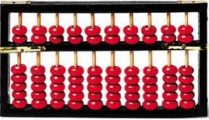
The earliest known tool for use in computation was the abacus, apparently it has been invented in Babylon about 2400 BC. Its original style of usage was by lines drawn in sand with pebbles. The more modern design is still used as calculation tool today (see the blog image).

The first recorded idea of using digital electronics for computing was the 1931 paper “The Use of Thyratrons for High Speed Automatic Counting of Physical Phenomena” by C. E. Wynn-Williams.

First Generation

(1940-1956) (from Webopedia)

The first computers used vacuum tubes for circuitry and magnetic drums for memory and were often enormous, taking up entire rooms. They were very expensive to operate and in addition to using a great amount of electricity, the first computers generated a lot of heat, which was often the cause of malfunctions.

First generation computers relied on machine language. This is the lowest-level programming language understood by computers to perform operations. They could only solve one problem at a time and it could take days or weeks to set-up a new problem. Input was based on punched cards and paper tape and output was displayed on printouts.

The UNIVAC and ENIAC computers are examples of first-generation computing devices. The UNIVAC was the first commercial computer delivered to a business client, the U.S. Census Bureau in 1951.

Second Generation

(1956-1963) (from Webopedia)

The transistor was invented in 1947. The transistor was far superior to the vacuum tube, allowing computers to become smaller, faster, cheaper, more energy-efficient and more reliable than their first-generation predecessors.
Second-generation computers still relied on punched cards for input and printouts for output.
Second-generation computers moved from cryptic binary machine language to symbolic, or assembly languages, which allowed programmers to specify instructions in words. High-level programming languages were also being developed at this time, such as early versions of COBOL and FORTRAN. These were also the first computers that stored their instructions in their memory, which moved from a magnetic drum to magnetic core technology.
The first computers of this generation were developed for the atomic energy industry.

Third Generation

(1964-1971) (from Webopedia)

Transistors were miniaturized and placed on silicon chips, called integrated circuits, which drastically increased the speed and efficiency of computers.
Instead of punched cards and printouts, users interacted with third generation computers through keyboards and monitors. The operating system allowed to share computing resources among many users (time sharing).
Computers (aka minicomputers) for the first time became accessible to a mass audience because they were smaller and cheaper than their predecessors (mainframes).

Fourth Generation

(1971-Present) (from Webopedia)

The microprocessor brought the fourth generation of computers (aka microcomputers), as thousands of integrated circuits were built onto a single silicon chip. What in the first generation filled an entire room could now fit in the palm of a hand.
The Intel 4004 chip, developed in 1971, located all the components of the computer – from the central processing unit and memory to input/output controls – on a single chip.

In 1981, IBM introduced its first computer for the home user and in 1984 Apple introduced the Macintosh. Microprocessors also moved out of the realm of desktop computers and into many areas of life as more and more everyday products.

As these small computers became more powerful, they could be linked together to form networks, which eventually led to the development of the Internet. Fourth generation computers also saw the development of GUIs, the mouse and hand-held devices.

Software history

Based on Wikipedia :

An outline (algorithm) for what would have been the first piece of software was written by Ada Lovelace in the 19th century for the planned Analytical Engine. However, neither the Analytical Engine nor any software for it, were ever created.

The first theory about software – prior to the creation of computers as we know them today – was proposed by Alan Turing in his 1935 essay “Computable numbers with an application to the Entscheidungsproblem” (decision problem).

The very first electronic computing devices were rewired in order to “reprogram” them !

The first time a stored-program computer held a piece of software in an electronic memory and executed it successfully was 11am, 21 June 1948, at the University of Manchester on the Small Scale Experimental Machine, also known as the “Baby” computer. It was written by Tom Kilburn, and calculated the highest factor of the integer 2^18 = 262,144. Starting with a large trial divisor, it performed division of 262,144 by repeated subtraction, then checked if the remainder was zero. If not, it decremented the trial divisor by one and repeated the process.

The first generation

The first generation of software for early stored program digital computers in the 1940s had its instructions written directly in machine language.
Machine language is the only programming language that the computer can understand directly without translation. It is a language made up of entirely 1s and 0s. The code must be written in accordance with the special characteristics of a given processor. Each type or family of processor has its own machine language.

The second generation

The first step in making software development easier and more efficient was the creation of assembly languages. They are also classified as low-level languages because detailed knowledge of hardware is still required. The first assembly language was developed in 1950 (Birkbeck assembler). Assembly languages use mnemonic operation codes and symbolic addresses in place of 1s and 0s to represent the operation codes.

Before Assembly can be executed by the computer, it must be translated into machine language. A language translator program called an assembler does this conversion. Assembly languages provide an easier and more efficient way to program than machine languages, while still maintaining control over the internal functions of a computer at the most basic level. The advantages of programming with assembly languages are that they produce programs that are efficient, use less storage, and execute much faster than programs designed using high-level languages.

The third generation

Where assembly languages, categorized as second generation programming languages, are machine-dependent, the third generation languages are machine independent and more programmer-friendly. Such languages are considered high-level because they are closer to human languages and further from machine languages. The main advantage of high-level languages over low-level languages is that they are easier to read, write and maintain. Ultimately, programs written in a high-level language must be translated into machine language by a compiler or interpreter.

Examples of early high level languages are FORTRAN (1957), ALGOL (1958) and COBOL (1960).

The fourth generation

A fourth-generation programming language (4GL) is a computer programming language envisioned as a refinement of the style of languages classified as third-generation programming language . Each of the programming language generations aims to provide a higher level of abstraction of the internal computer hardware details, making the language more programmer-friendly, powerful and versatile.
The fourth generation programming language can be typified by operating more with large collections of information at once and problem solving, rather than focusing on just bits and bytes.
Languages claimed to be 4GL may include support for database management, report generation, mathematical optimization, GUI development or web development.

Examples :
Santa Fe railroad used MAPPER (1968) to develop a system, in a project that was an early example of 4GL, rapid prototyping and programming by users. The idea was that it was easier to teach railroad experts to use MAPPER than to teach programmers the “intricacies of railroad operations”.

One of the early languages that had 4GL properties was Ramis developed by Gerald C. Cohen at Mathematica, a mathematical software company. Cohen left Mathematica and founded Information Builders to create a similar reporting-oriented 4GL, called FOCUS.

Later 4GL types are tied to a database system (SQL – 1972) and are far different from the earlier types in their use of techniques and resources.

TeX is a typesetting system written by Donald E. Knuth. He developed the first version of TeX in 1978 to deal with revisions to his book series “The Art of Computer Programming”. The idea of TeX proved popular and Knuth produced a second version (in 1982) which is the basis of what we use today.

Operating systems

On the first computers without an operating system, every program needed the full hardware specification to run correctly and perform standard tasks.
The growing complexity of hardware and application programs eventually made operating systems a necessity for everyday use. Resident background programs, capable of managing multistep processes, were often called monitors or monitor-programs before the term “operating system” established itself.

In technical and development circles, the old restricted sense of an OS (monitor) persists because of the continued active development of embedded operating systems for all kinds of devices like hand-held gadgets up to industrial robots and real-time control-systems. An embedded operating systems in a device today is not so far from its ancestor, the monitor.

The true descendant of the early monitors is what is now called the “kernel“.

1956 the first batch operating system used for real work was GM-NAA I/O, produced by General Motors’ Research division for its IBM 704. Most other early operating systems for IBM mainframes were also produced by customers.

1961 Time sharing CTSS for IBM 7094

1965 Multi programming Eindhoven University of Technology

Types of OS :
– Batch
– Time sharing (multi user)
– Multi programming / tasking
– Real time
– Single user

Parallel computing

• One machine multiple CPUs

Basically, parallel computing is the simultaneous use of multiple CPUs to solve a computational problem. A problem/program is broken into parts that can be solved/executed concurrently. Each part is further broken down to a series of instructions. Instructions from each part execute simultaneously on different CPUs. An overall control/coordination mechanism is employed.

In parallel computing, all processors may have access to a shared memory to exchange information between processors. On the other hand, in distributed computing (like cluster-, grid- and cloud- computing) each processor has its own private memory.

Parallel computing began to proliferate in using parallel CPUs at the high end and multi-core architectures at the low-end. Parallel computing is much better suited for modeling, simulating and understanding complex, real world phenomena than serial computing.

Modern computers, even laptops, are parallel in architecture with multiple cores. Parallel software is specifically intended for parallel hardware with multiple CPUs/cores.

Parallel computing is the base for modern supercomputers.

From Wikipedia :

Burroughs Corporation introduced the D825 in 1962, a four-processor computer that accessed up to 16 memory modules through a crossbar switch.

In 1969, company Honeywell introduced its first Multics system, a symmetric multiprocessor system capable of running up to eight processors in parallel.

Cluster computing

(distributed computing)

• multiple machines (local)
• connected via fast LAN
• usually same HW and OS
• clustering middleware

From Wikipedia :

A computer cluster is a group of linked computers working together closely, so that in many respects they form a single computer. The computers of a cluster are usually connected to each other through fast local area networks. Clusters are usually deployed to improve performance and/or availability compared to the one provided by a single computer, while typically being much more cost-effective than single computers of comparable speed or availability.

The first production system designed as a cluster was the Burroughs B5700 in the 1971. This allowed up to four computers, each with either one or two processors, to be tightly coupled to a common disk storage subsystem in order to distribute the workload. Unlike standard multiprocessor systems, each computer could be restarted without disrupting overall operation.

The first commercial loosely coupled clustering product was Datapoint Corporation’s “Attached Resource Computer” (ARC) system, developed in 1977, and using ARCnet as the cluster interface.
Clustering per se did not really take off until Digital Equipment Corporation (DEC) released their VAXcluster product in 1984.

Cluster computing is used in modern supercomputers.

Grid computing

(distributed computing)

• multiple machines (multiple locations)
• connected via Internet or private (remote) network
• usually heterogeneous HW and OS
• grid middleware

Multiple independent computers act like a “grid”, because they are composed of resource nodes not located within a single administrative domain.

Grids started off in the mid-90s to address large-scale computation problems, then only solvable by using supercomputers or dedicated clusters. The major motivation was that these high performance
computing resources were expensive and hard to get access to. The starting point was to use federated resources that could comprise compute, storage and network resources from multiple geographically distributed institutions.

Grid computing provides a framework (grid middleware) for exploiting under utilized resources and thus has the possibility of substantially increasing the efficiency of resource usage.
In a grid, one large job is divided into many small portions and executed on multiple machines.

One of the benefits of a grid is to better balance resource utilization. An organization may have occasional unexpected peaks of activity that demand more resources. During such peaks, an application can be moved to under-utilized machines.

Grid computing is the father/mother of cloud computing.

Cloud computing

(distributed computing)

• multiple machines (multiple locations)
• connected via Internet
• usually heterogeneous HW and OS
• cloud middleware

Users of the cloud only need to be concerned with the computing service being asked for, as the underlying details of how it is achieved are hidden. This method of distributed computing is done through pooling all computer resources together and being managed by the cloud middleware.

The services being requested of a cloud are not limited to using web applications, but can also be IT management tasks such as requesting of systems, a software stack or a specific web appliance.

Cloud computing vs. Grid computing

While grid computing also offers a similar facility for computing power, cloud computing isn’t restricted to just that.
The cloud is intended to allow the user to access services without investing in the underlying architecture.

Grid computing uses sprawling networks meant to handle a limited number of big tasks over the Internet.
Cloud computing uses large clusters of computers that can be accessed over the Internet to handle smaller processing tasks from many sources.